Mapping the Second Industrial Revolution
Mapping the 2nd Industrial Revolution
Complexity Science Hub
Introduction
- 19th Century: rapid technological change
- Creative destruction: destroyed jobs, created new jobs (Acemoglu & Restrepo 2019)
- New Jobs: have been vital (Autor et al, 2025; Kalyani et al 2025)
- 60% of the jobs that employ Americans today did not exist in the 1950s.
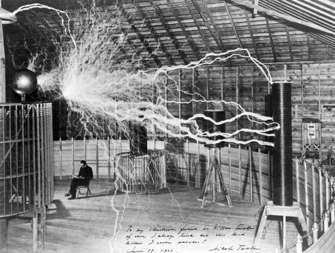
This Paper: Quantify Jobs Lost & Jobs Created in 2nd IR
- Aim: Understand how and where job creation mapped on to job loss
- Problem: No systematic quantitative record of job creation and loss in Victorian Britain
- Solution: Generate “micro-occupation” data. 800 industries → 10,000 micro-occupations.
- Quantify: new and declining occupations in Britain 1851–1911
History: 2nd Industrial Revolution
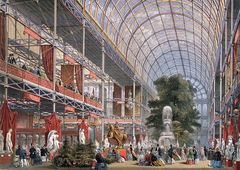
- 1851: Crystal Palace — Workshop of the World
- 1870s: Britain — shift to a new phase of industrialization.
- Traditional crafts sectors start declining
- Vast numbers of new jobs emerging: electricians, engineers, railway workers
History: British Census
- 1753 Thomas Potter: bill introduced to Parliament. Army, emigration to the colonies, burden of the poor law. Population growth.
- 1801–1831: Parish (township) register aggregates
- 1841–1921: Individual Level
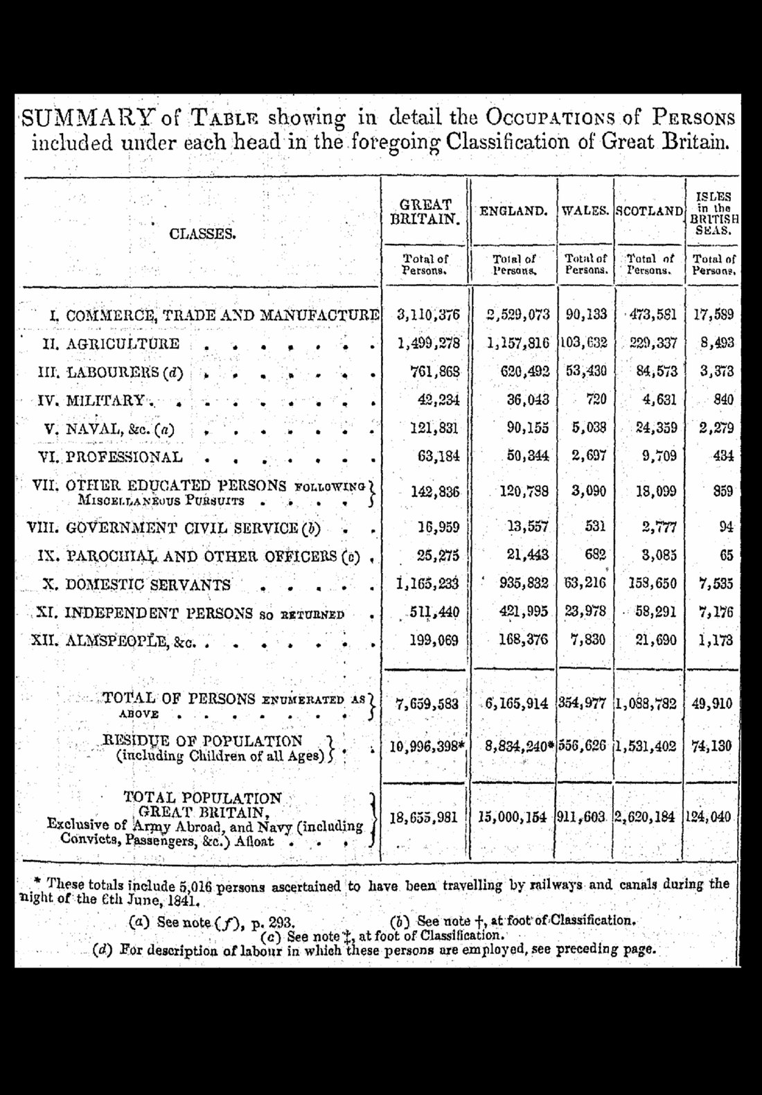
History: British Census Classification Schema
- 1841: First individual level census
- 1851: 18 orders, 90 sub-orders
- 1861: “The classification of 1851 has been entirely revised”. Dress goes from Services to Textiles. Animal/Vegetable matter go.
- By 1901: 23 Orders, substantial changes in sub-orders
Data: The Integrated Census Microdata Project (ICeM)
- Decennial English census data from 1851 to 1921 (excluding 1871)
- 220 million individual level census records, digitized
- Occupation: at industry level

Data Construction 1: “Task” Occupation
| Industry Code | Occupation — Original Strings | New Variable: “Task” |
|---|---|---|
| 663 (Bootmaker) | CORDWAINER | Cordwainer |
| 663 (Bootmaker) | BOOT & SHOE MAKER | Maker |
| 663 (Bootmaker) | BOOT AND SHOE BINDER | Binder |
| 663 (Bootmaker) | BOOT & SHOE RIVETTER | Rivetter |
| 663 (Bootmaker) | SEWING MACHINIST | Sewing Machinist |
The table shows examples of original occupation strings from Census records and their corresponding new variable “Task”. I assign 97% of them to “Task”.
Data Construction 1: “Task” Occupation
Every spelling of tailor found in the census strings:
Data Construction 2: Census Linking
- Context: Census linking is indispensable
- Concern: False positives pose threat to inference:
- Migration: O'Grada et al. (2025), 68–77% vs 14%
- Occupation: Helgertz et al. (2023)
- Problem: Without ground truth, how to check?
- Solution: Leverage statistical regularities of false matches: litmus test
Methods
1. Overview
- 6.5 million unique strings describing occupation
- Around 800 occupation codes
- The census gives us some help: enumerators worked to written instructions
- Most important job first
- second instruction — to come
2. Three Main Challenges
3. AI-Assisted Human Labeling
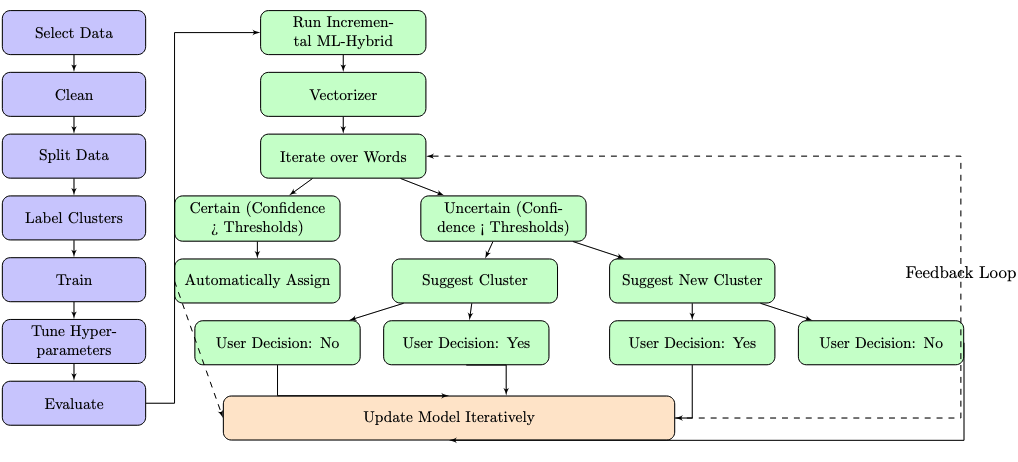
- load and count
- cleaning
- top 100
- draft from the dictionary
- magnet
- LLM confirms
- priority rules
- fragment + industry-only
- residue pass
- deliverables — five files
4. Current Pipeline
5. Output
| string | records | cum % | task 1 | task 2 | product |
|---|---|---|---|---|---|
| SHOEMAKER | 204,192 | 15.8% | shoemaker | — | shoe |
| SHOE MAKER | 168,665 | 28.9% | shoemaker | — | shoe |
| BOOT MAKER | 95,594 | 36.3% | bootmaker | — | boot |
| CORDWAINER | 77,458 | 42.3% | cordwainer | — | — |
| BOOTMAKER | 50,830 | 46.2% | bootmaker | — | boot |
| SHOE BINDER | 33,703 | 48.9% | binder | — | shoe |
| SHOE FINISHER | 31,231 | 51.3% | finisher | — | shoe |
| BOOT MACHINIST | 28,036 | 53.4% | machinist | — | boot |
| BOOT & SHOE MAKER | 24,391 | 55.3% | bootmaker | shoemaker | boot |
| BOOT FINISHER | 24,324 | 57.2% | finisher | — | boot |
| BOOT REPAIRER | 23,769 | 59.1% | repairer | — | boot |
| SHOE MACHINIST | 18,997 | 60.5% | machinist | — | shoe |
| BOOT BINDER | 17,434 | 61.9% | binder | — | boot |
| BOOT CLOSER | 15,216 | 63.1% | closer | — | boot |
| SHOE RIVETTER | 14,889 | 64.2% | rivetter | — | shoe |
| SHOE FITTER | 12,722 | 65.2% | fitter | — | shoe |
| BOOT AND SHOE MAKER | 12,056 | 66.1% | bootmaker | shoemaker | boot |
| BOOT FITTER | 10,400 | 66.9% | fitter | — | boot |
| SHOE CLICKER | 9,089 | 67.6% | clicker | — | shoe |
| CLICKER | 8,955 | 68.3% | clicker | — | — |
Descriptive Evidence
1. Occupational Orders over Time
2. Orders ranked by growth, 1851–1911
Showing the growth in different sectors of the economy over the period. Sectors shown in blue are growing more rapidly than average population growth.
3. Occupational Industries: Growth and Decline
Showing growth by industry over the period. Note that the extreme outliers are primarily in industries which were very small or non-existent in 1851.
Population doubled over the period: any industry growing more than 100% outpaced population growth, industries which grew less lagged.
4. Micro-Occupations: Growth and Decline
Each industry is itself made up of many different jobs — micro-occupations.
New Evidence
1. Map of specific new jobs
Where did specific new occupations emerge across the country?
New jobs of the 19th century
Ranked by number of workers, 1911.
| Occupation | Workers, 1911 |
|---|---|
| Electrician | 55,447 |
| Motor driver | 44,947 |
| Typist | 41,927 |
| Bicycle maker | 33,461 |
| Telegraph | 33,129 |
| Telephonist | 19,230 |
| Photographer | 17,134 |
| Asphalter | 1,612 |
| Anaesthetist | 353 |
| X-ray operatorAlso known as… radiographer · skiagraphist · roentgenologist · x-rayist · x-ray man (even railway xrayman) · x-ray attendant · x-ray photographer | 77 |
2. Mapping of management jobs
An initial mapping of the rise of management jobs in the UK, by county.
3. Map of mechanization
An initial mapping of the emergence of new technologies in the UK, by county.
Mechanization rises on both measures. In share and absolute numbers, by 1911 there are 1.5 million more people working with machines.
4. Mapping of the apprenticeship system
The apprenticeship system declines everywhere between 1851–1911. The decline is more rapid after 1881. Less urban areas seem to retain more of the system than elsewhere.
But this is a decline in share, not in absolute numbers. Summed across the three roles, the system actually grows slightly — from about 252,000 in 1851 to about 261,000 in 1911, a net rise of roughly 9,000. Apprentices themselves increase substantially, by almost 90,000; the real decline is among journeymen (down about 65,000) and masters.
Total Participation
Role Breakdown
Results
1.1. Measuring displacement
Picking out an outlier
- I run this regression 231 times.
- shows how much an occupation’s exit rate moves vis-à-vis the average.
1.2. Who was displaced
1.3. Did contraction push workers out?
1.4. Or did it stop new ones coming in?
1.5. More unusual on exit, or on entry?
Each occupation is ranked twice against the same universe of 235 large male occupations. Once on exit rate increasing, once on how much entry collapsed.
- Everything is extreme on entry. All 18 sit above the 71st percentile of entry collapse.
- Exit is what separates them.
Results
2.1. Which industries had managers?
- In 1851, seven occupations held half the managers.
- By 1901 it took thirty-one.
- Supervision spread out across the economy.
2.2. How many managers?
- 25,000 managers in 1851.
- 282,000 by 1911, an elevenfold rise.
- More supervisors, spread over more trades.
2.3. Where did managers come from?
2.4. Fathers’ occupations in occupation space
2.5. Fathers’ occupational status
2.6. Where the new bootmaking jobs were
2.7. Growing up in a mechanizing county
Were boys raised in Leicestershire or Northamptonshire more likely to become bootmaking foremen thirty years later?
- 0.45pp more likely to become bootmaking foremen.
- Unchanged with age and cohort controls.
- All boys, so entry and advancement together — not promotion within the trade.
Results
3.1. Sons entering their father’s occupation
3.2. Where the new bootmaking jobs were
3.3. Comparing brothers
- Family FE holds parents, place and upbringing constant, and therefore comparison is between brothers.
- is the gap between the son who followed his father and the son who did not.
- is how much wider that gap is where the trade was collapsing.
3.4. The cost of persistence: children under 18
| Bootmaker sons | Carpenter sons — placebo | |||
|---|---|---|---|---|
| 1851–1881 | 1861–1891 | 1851–1881 | 1861–1891 | |
| Entered the trade | 0.448*** | 0.261* | −0.011 | 0.659** |
| (0.107) | (0.137) | (0.270) | (0.243) | |
| × Decline county | −0.240* | −0.220 | 0.351 | −0.348 |
| (0.137) | (0.161) | (0.276) | (0.256) | |
| Total gap in Decline | 0.208** | 0.041 | 0.340*** | 0.312*** |
| [0.082] | [0.096] | [0.060] | [0.073] | |
| Observations | 3,329 | 2,816 | 3,356 | 2,920 |
| R2 | 0.488 | 0.487 | 0.468 | 0.499 |
- Bootmaker sons had more children than their brothers, and Decline takes about half of that back.
- No carpenter interaction is distinguishable from zero.
3.5. Age at marriage in old and new bootmaking
Conclusion
- From roughly 800 industries to about 10,000 micro-occupations.
- Micro-occupations are necessary to track the emergence of new work and the decline of older jobs.
- Rise of management jobs and factory work.
- Decline of the apprenticeship system, in terms of shares. In absolute numbers, it increases by about 9,000.
- Implications: how society absorbs technological shocks; who gets the new jobs.
- Next steps: finalise boundaries and definitions of new jobs.
Appendix
1. The shape of the workforce: Orders, sub-Orders, and occupations
Every occupation nests inside a sub-Order, and every sub-Order inside one of the 22 Orders. The circles below pack that whole structure, with each circle's area proportional to its 1911 workforce. Click any bubble to zoom in; click the background to zoom back out.
2. Changing Taxonomies: Census Waves 1851–1911
The grey treemap is the 1911 classification: Orders, their sub-Orders and the occupations within them. Hovering an occupation in an earlier census lights up the others it was lumped with — the more scattered, the more that census cut across the modern Orders.
3. Migration within Orders, 1851 → 1861
Zoom in one level. Even within a single Order, the census kept reorganising. Here the 22 Orders stay fixed as the outer bubbles, and inside each one the occupations are grouped by their real census category for the chosen year. Flip between 1851 and 1861 to watch occupations split apart, merge together, or reshuffle within their Order. Unchanged occupations stay grey.